

3.Function

3. 활성화 함수

sigmoid 함수

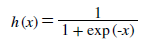
sigmoid 함수는 어떠한 input에 대하여 0 ~ 1 사이의 output을 내는 함수이다. 신경망에서는 활성화함수로 sigmoid 함수를 이용해 신호를 변환하고 그 변환된 신호를 다음 뉴런 에 전달한다.

퍼셉트론과 신경망의 주된 차이는 활성화 함수이고 그 밖에 여러층으로 이어지는 구조와 신호를 전달하는 방법은 기본적으로 앞에서 봤던 perceptron 과 같다.

---

계단 함수

import numpy as np

def step_func(x):
    y = x > 0
    print(y)
    return y.astype(np.int)


arr = np.array([[-1.0, 2.0], [0.0, 2.0]])
step_func(arr)

[[False  True]
 [False  True]]





array([[0, 1],
       [0, 1]])

위는 numpy array로 선언된 변수를 계단 함수에 넣어 결과를 얻어낸 것이다. x로 각 행렬 원소들이 들어가게 되고 각 행렬의 shape에 맞춰 결과값이 나오게 된다.

처음 부등호 연산을 시행할 때는 단순히 bool 형태가 나오게 되지만 이후 astype() 메소드를 통해서 해당 부분을 int 형으로 바꿔주게 된다. 따라서 결과값은 integer 형태를 얻을 수 있다.

그래프

계단함수의 그래프를 matplotlib 라이브러리를 이용해 그릴 수 있다.

import numpy as np
import matplotlib.pylab as plt

def step_func(x):
    return np.array(x > 0, dtype = np.int)


x = np.arange(-5.0, 5.0, 0.1)
# print(x.shape)

y = step_func(x)

plt.plot(x, y)
plt.ylim(-0.5, 1.5)
plt.show()

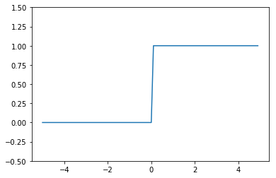
위의처럼 계단함수의 그래프는 특정값 이상일 때 1 or 0의 값을 나타내게 된다.

sigmoid 함수 구현

sigmoid는 계단함수보다 훨씬 더 유연한 형태를 띠고 있다.

import numpy as np
import matplotlib.pylab as plt

def sigmoid(x):
    return 1 / (1 + np.exp(-x))

x = np.arange(-5.0, 5.0, 0.1)
y = sigmoid(x)

# print(x.shape, y.shape)

plt.plot(x, y)
plt.ylim(-0.1, 1.1)
plt.show()

<Figure size 640x480 with 1 Axes>

비선형 함수

계단 함수와 sigmoid 두 함수는 비선형 함수 이다. 신경망을 구성할 때는 활성화 함수로 비선형 함수를 사용해야 한다. 이는 선형함수를 사용하게 된다면 각 weight 값이 망의 깊이가 깊어짐에 따라 의미가 없어지기 때문이다.

ReLU 함수

sigmoid, 계단 함수등을 설명했지만 최근에는 좀 더 다른 함수를 쓴다. ReLU 함수는 입력이 0을 넘으면 비례해서 출력을 해주고 0 이하라면 0을 출력해주는 함수이다.

def ReLU(x):
    return np.maximum(0, x)


x = np.arange(-5.0, 5.0, 0.1)
ReLU(x)

array([0. , 0. , 0. , 0. , 0. , 0. , 0. , 0. , 0. , 0. , 0. , 0. , 0. ,
       0. , 0. , 0. , 0. , 0. , 0. , 0. , 0. , 0. , 0. , 0. , 0. , 0. ,
       0. , 0. , 0. , 0. , 0. , 0. , 0. , 0. , 0. , 0. , 0. , 0. , 0. ,
       0. , 0. , 0. , 0. , 0. , 0. , 0. , 0. , 0. , 0. , 0. , 0. , 0.1,
       0.2, 0.3, 0.4, 0.5, 0.6, 0.7, 0.8, 0.9, 1. , 1.1, 1.2, 1.3, 1.4,
       1.5, 1.6, 1.7, 1.8, 1.9, 2. , 2.1, 2.2, 2.3, 2.4, 2.5, 2.6, 2.7,
       2.8, 2.9, 3. , 3.1, 3.2, 3.3, 3.4, 3.5, 3.6, 3.7, 3.8, 3.9, 4. ,
       4.1, 4.2, 4.3, 4.4, 4.5, 4.6, 4.7, 4.8, 4.9])

위와 같은 형식으로 ReLU 함수를 선언할 수 있다.

---

다차원 배열의 계산

다차원 배열 선언과 계산

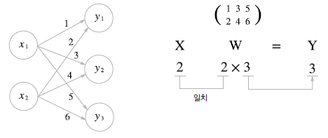
1 차원 배열과 2차원 배열을 np.array 함수를 통해서 선언할 수 있다.

dim1_arr = np.array([1, 2, 3])
dim2_arr = np.array([[1, 2, 3], [10, 20, 30]])

print(dim2_arr.shape)

A = np.dot(dim2_arr, dim1_arr)
print(dim2_arr.shape)
print(dim1_arr.shape)

print(A)
print(A.shape)

(2, 3)
(2, 3)
(3,)
[ 14 140]
(2,)

이러한 배열들은 위와 같은 연산들이 가능하다. 그리고 신경망에서도 이러한 행렬의 곱을 사용할 수 있다.

위와 같은 방식으로 다층 신경망을 구현할 수도 있다.

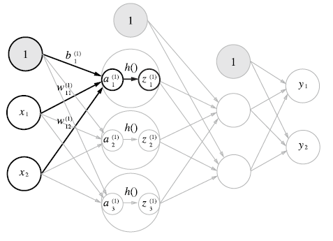
각 layer마다 bias 값을 더하면서 각 계층의 퍼셉트론에 활성화함수가 적용된

import numpy as np
import tensorflow as tf

def sigmoid(x):
    return 1 / (1 + np.exp(-x))

X = np.array([10, 20])
W1 = np.array([[1, 2, 3, 4], [10, 20, 30, 40]])
b1 = 1

result = np.dot(X, W1)

print(result)
print(result.shape)

X = np.array([[10, 20]])
W1 = np.array([[1, 2, 3, 4], [10, 20, 30, 40]])
b1 = 10

result = np.matmul(X, W1)

print(result)
print(result.shape)

[210 420 630 840]
(4,)
[[210 420 630 840]]
(1, 4)

위는 matmul과 dot을 구분지어서 결과를 낸 것이다. 각각의 결과를 보면 matmul의 경우 행렬의 곱셈을 나타내는 것으로 두 개 전부 data의 값은 같지만 matmul의 경우 하나의 벡터결과로 나타나게 되는것을 알 수 있다.

다층 신경망

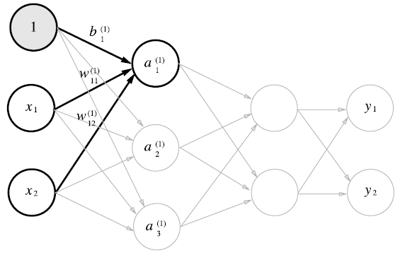
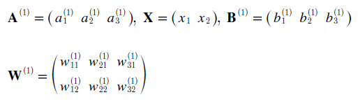
각 신경망의 weight 및 뉴런들은 위와 같이 도식화가 가능하다. 그리고 행렬의 곱을 이용해서 식을 간소화시킬 수 있다. 각 행렬들은 다음과 같이 나타나게 된다.

이를 numpy 모듈을 사용해서 구현할 수 있다.

import numpy as np
import tensorflow as tf

def sigmoid(x):
    return 1 / (1 + np.exp(-x))

# layer1 np.dot process
X = np.array([1, 2])
W1 = np.array([[0.1, 0.2, 0.3], [0.5, 0.6, 0.3]])
b1 = 1

# layer 1 result; np.dot
L1 = np.dot(X, W1) + b1
print('[] L1 shape: ', L1.shape)

# layer 2 np.dot process
W2 = np.array([[0.1], [0.2], [0.3]])
b2 = 0.1

print(sigmoid(L1))

# np.matmul process
X = np.array([[1, 2]])
W1 = np.array([[0.1, 0.2, 0.3], [0.5, 0.6, 0.3]])
b1 = 1

# layer 1 result; np.matmul
L1 = np.matmul(X, W1) + b1

print('[] np.matmul: ', L1)
print('[] np.matmul shape: ', L1.shape)

print(sigmoid(L1))

[] L1 shape:  (3,)
[0.89090318 0.9168273  0.86989153]
[] np.matmul:  [[2.1 2.4 1.9]]
[] np.matmul shape:  (1, 3)
[[0.89090318 0.9168273  0.86989153]]

layer1을 np.dot, np.matmul을 이용해서 구현한 상태이다. 각 결과를 보면 데이터는 같지만 shape가 다르게 나오는 것을 알 수 있다. 그리고 활성화 함수를 은닉층의 뉴런에 배치해 실제 딥러닝 프레임워크의 layer 1을 표현하였다.

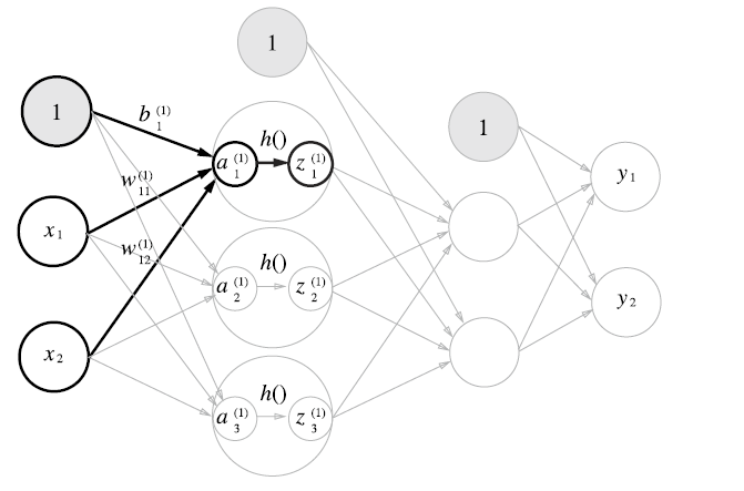
code는 입력층 부분에서 layer1으로 넘어가는 부분을 표현하였기에 이 후 행렬 값만 제대로 맞춰서 여러 layer를 가진 딥 러닝 구조를 만들 수 있다.

import numpy as np
import tensorflow as tf

def sigmoid(x):
    return 1 / (1 + np.exp(-x))

def check(x):
    print('[] shape: ', x.shape)

# np.dot network init
def dot_net_init():
    net = {}
    net['W1'] = np.array([[0.3, 0.1], [0.6, 0.1], [0.5, 0.2]])
    net['b1'] = np.array([1, 1])
    net['W2'] = np.array([[0.1, 0.1, 0.5], [0.8, 0.3, 0.2]])
    net['b2'] = np.array([0.1, 0.4, 0.5])
    net['W3'] = np.array([[0.3], [0.1], [0.4]])
    net['b3'] = np.array([0.5])
    return net

def dot_process(X, net):
    L1 = np.dot(X, net['W1']) + net['b1']
    temp = sigmoid(L1)
    L2 = np.dot(temp, net['W2']) + net['b2']
    temp = sigmoid(L2)
    L3 = np.dot(temp, net['W3']) + net['b3']

    return sigmoid(L3)

def matmul_process(X, net):
    # for matrix operation
    X = np.array([X])

    L1 = np.dot(X, net['W1']) + net['b1']
    temp = sigmoid(L1)
    L2 = np.dot(temp, net['W2']) + net['b2']
    temp = sigmoid(L2)
    L3 = np.dot(temp, net['W3']) + net['b3']

    return sigmoid(L3)

def main():
    # input matrix: (3,); np. dot process
    X = np.array([1, 1, 1])

    # init neural network
    net = dot_net_init()

    # np.dot process start
    result = dot_process(X, net)
    print('[] dot process result: ', result)
    print('[] dot result shape: ', result.shape)

    # np.matmul process start
    result = matmul_process(X, net)
    print('[] matmul process result: ', result)
    print('[] matmul result shape: ', result.shape)

if __name__ == '__main__':
    main()

[] dot process result:  [0.74614674]
[] dot result shape:  (1,)
[] matmul process result:  [[0.74614674]]
[] matmul result shape:  (1, 1)

위에서는 np.dot, np.matmul을 이용해서 3개의 layer로 이뤄진 딥 러닝을 구성해보았다

L1: 2 L2: 3 L3: 1

위와 같이 각 뉴럴이 구성되어 있으며 행은 input의 개수, 열은 output의 개수로 맞춰주면 되는 것을 알 수 있다. 그리고 각 계층 별로 result 값이 나오면 활성화함수 (sigmoid, ReLU) 를 사용해서 값을 재정비하고 그 이후 그 값을 다음 layer에 넣어줘야 한다.

---

출력층 설계

기계 학습 문제에서는 결과를 분류, 회귀 로 나누게 된다. 분류는 데이터가 어느 class에 소속하느냐를 구분하는 문제이고 회귀는 입력데이터에서 연속적인 수치를 예측하는 문제이다.

Softmax 함수

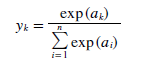
softmax 함수는 식은 분류에서 사용한다. n은 출력층의 뉴런 수 yk는 그 중 k번 째 출력 임을 뜻한다. softmax 함수를 쓰는 이유는 결과를 확률 값으로 해석하려 하기 위함이다.

이는 각 뉴런들의 활성화 함수와는 달리 최종 출력계층에서 작용하여 각 결과를 확률로 보내는데 사용된다.

import numpy as np

def softmax(x):
    exp_x = np.exp(x)
    print(exp_x)
    s = np.sum(exp_x, 0)

    y = exp_x / s

    return y

test = np.array([1, 2, 3])
print(softmax(test))

[ 2.71828183  7.3890561  20.08553692]
[0.09003057 0.24472847 0.66524096]

위의 softmax는 구현이 잘 되지만 기본적으로 사용되는 exp 함수는 지수함수로 나타나기 때문에 작은 값에도 결과값은 아주 큰 값이 나올 수 있다. 그렇다면 NaN이라는 결과가 나오게 된다.

X = np.array([1000, 1001, 2000])

softmax(X)

[inf inf inf]


C:\Users\pulpan92\Anaconda3\envs\machine\lib\site-packages\ipykernel_launcher.py:4: RuntimeWarning: overflow encountered in exp
  after removing the cwd from sys.path.
C:\Users\pulpan92\Anaconda3\envs\machine\lib\site-packages\ipykernel_launcher.py:8: RuntimeWarning: invalid value encountered in true_divide






array([nan, nan, nan])

이를 방지하려면 input으로 들어가는 행렬 중 가장 큰 원소를 뺀 후 그 값을 softmax에 넣으면 된다.

import numpy as np

def softmax(X):
    maxnum = np.max(X)
    print(X - maxnum)
    exp_x = np.exp(X - maxnum)
    print(exp_x)
    s = np.sum(exp_x, 0)

    y = exp_x / s

    return y


X = np.array([1010, 1000, 990])

print(softmax(X))

[  0 -10 -20]
[1.00000000e+00 4.53999298e-05 2.06115362e-09]
[9.99954600e-01 4.53978686e-05 2.06106005e-09]

softmax 함수의 가장 큰 특징은 모든 확률의 값이 1인 것이다. 따라서 출력층에서 softmax를 거쳐 나온 결과물들을 확률로 해석할 수 있다.

---

손글씨 인식

MNIST dataset

손글씨 숫자 이미지 집합을 나타낸 것이다. 이는 총 train image 60000장, test image 10000장이 있고 각각의 label이 따로 있다.

from tensorflow.examples.tutorials.mnist import input_data

mnist = input_data.read_data_sets('MNIST_data', one_hot = True)
batch = mnist.train.next_batch(100)

Extracting MNIST_data\train-images-idx3-ubyte.gz
Extracting MNIST_data\train-labels-idx1-ubyte.gz
Extracting MNIST_data\t10k-images-idx3-ubyte.gz
Extracting MNIST_data\t10k-labels-idx1-ubyte.gz

위는 tensorflow module에서 train의 각 100개의 image와 label을 갖고오게 된다. batch[0]은 image, batch[1]은 label 데이터들이 담겨져 있다.

import numpy as np
from tensorflow.examples.tutorials.mnist import input_data

def get_data():
    mnist = input_data.read_data_sets('MNIST_data', one_hot = True)
    batch = mnist.train.next_batch(10000)

    return batch


def init_net():
    net = {}
    net['W1'] = np.array

def main():
    mnist = get_data()
    print(mnist[0][1].shape)


if __name__ == '__main__':
    main()

Extracting MNIST_data\train-images-idx3-ubyte.gz
Extracting MNIST_data\train-labels-idx1-ubyte.gz
Extracting MNIST_data\t10k-images-idx3-ubyte.gz
Extracting MNIST_data\t10k-labels-idx1-ubyte.gz
(784,)

댓글